Linear Regression with Scikit-Learn

A quick guide to implementing Linear regression in Python

Author Fortune Uwha, Turing College learner

Introduction

Linear regression is the simplest machine learning algorithm to get started with, making it perfect for beginners. In fact, it’s so easy that you can basically get started with machine learning today — like, right now. So looking to begin your machine learning journey? This is a good start.

What is Linear Regression?

The aim of linear regression is to identify how the independent variable(explanatory variable) influences the dependent variable(response variable).

You can think of independent and dependent variables in terms of cause and effect. An independent variable is the variable you think is the cause, while a dependent variable is the effect. For example, in an exam context, the number of questions answered correctly results in a passing grade. So questions answered correctly(q) is the cause(independent variable), then the passing grade(p) is the effect(dependent variable).

Linear Regression explained using sample Dataset

To share my understanding of the concept and techniques I know, we’ll take an example of the student performance dataset which is available on UCI Machine Learning Repository and try to predict grades based on students behaviour and students past grades.

For our purposes, building a linear regression model will involve the following five steps:

Step 1: Importing the libraries/dataset

Step 2: Data pre-processing

Step 3: Splitting the dataset into a training set and test set

Step 4: Fitting the linear regression model to the training set

Step 5: Making predictions

1. Importing the libraries/dataset

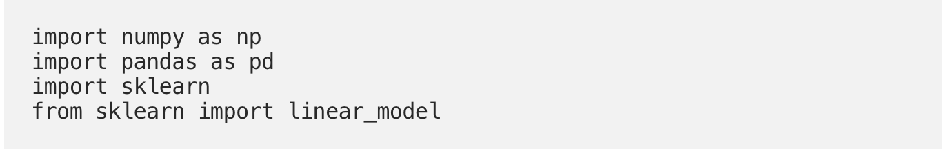
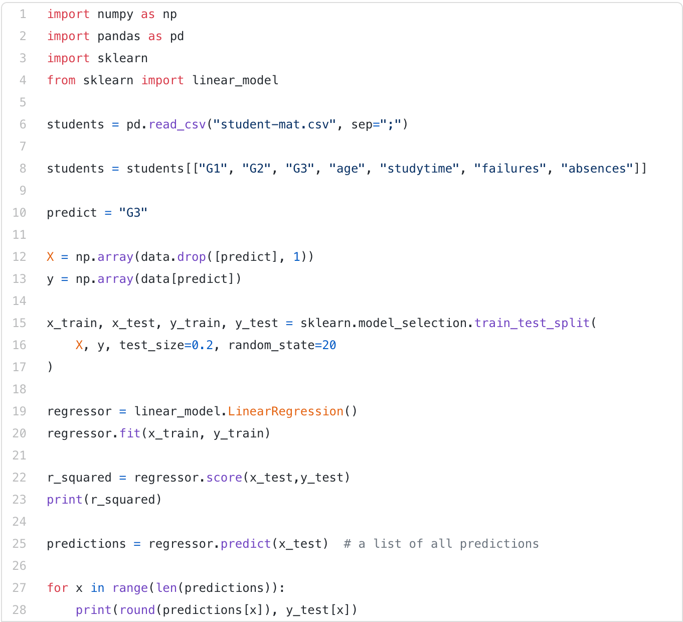
We will begin with importing the dataset using pandas (sadly, not these 🐼) and also import other libraries such as NumPy and sklearn.

Note: Whatever inferences I could extract, I’ve mentioned with bullet points.

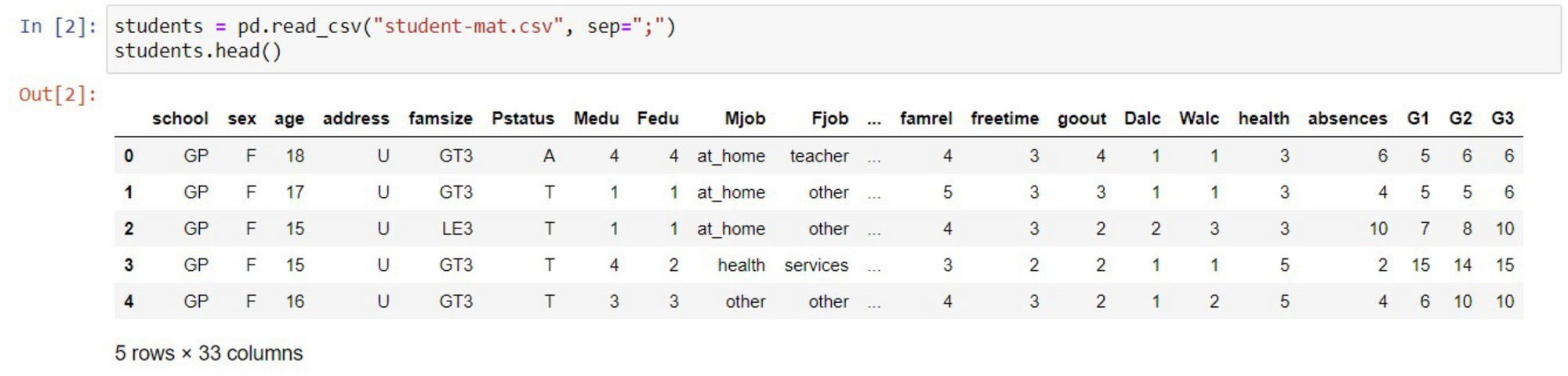
* Original data is separated by semicolons delimiter, we need to do sep=”;”.

* The students.head() shows attributes about the first 5 students in our data frame.

2. Data Preprocessing

Since we have so many attributes and not all are relevant, we need to select the ones we want to use. We can do this by typing the following. Feel free to try out different attributes and the effect on the model at the end of this walk-through.

NB: Remember you can see a description of each attribute here.

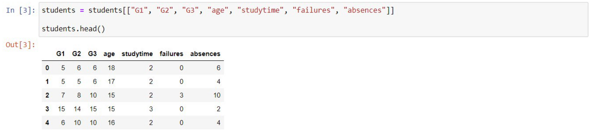
* Based on these attributes we want to predict the student’s final grade(G3). Our next step is to divide the data into X “Features”(explanatory variables) and y, “target”(response variable).

3. Splitting the dataset into a training set and test set

Why is it necessary to perform splitting?

We want our algorithm to learn correlations in our data and then to make predictions based on what it learned. Splitting the data into two different sets ensures that our linear regression algorithm doesn’t overlearn.

Think of this scenario:

Let’s say you teach a child to multiply by letting the kid train on a small multiplication table, i.e. everything from 1*1 to 9*9. Next, you test whether the kid is able to perform the same multiplications. The result is a success. The kid gets it right almost every time.

The problem? You don’t know if the kid understands multiplication at all, or has simply memorized the table! So what you would do instead is test the kid on multiplications like 10*12, that is outside of the table.

This is exactly why we need to test machine learning models on *unseen *data. We check whether the predictions made by the model on the test set data matches what was given in the dataset. If it matches, it implies that our model is accurate and is making the right predictions. Otherwise, we have no way of knowing whether the algorithm has learned a generalizable pattern or has simply memorized the training data.

We can split this dataset by typing out the following:

There is no ideal ratio for the train: test split. But for the purpose of this tutorial,we could use the 80: 20 split. i.e 80% as training and 20% as a testing set. Of course, feel free to use other ratios e.g 70:30, 90:10 e.t.c

4. Fitting the linear regression model to the training set

Now that our data is ready, our first step is to fit the simple linear regression model to our training set. To do this, we will call the fit method — function to fit, the regressor to the training set.

We need to fit X_train (training data of matrix of features) into the target values(y_train). Thus, the model learns the correlation and learns how to predict the dependent variable based on the independent variables.

5. Making Predictions

To see how well our algorithm performed on our test data, we will use the metric 𝑅². 𝑅² score shows how well the regression model fits the observed data. For example, an r-squared of 70% reveals that 70% of the data fit the regression model. Generally, a higher r-squared indicates a better fit for the model. However, it is important to note that this is not always the case that a high r-squared is good for the regression model.

For this specific data set a score of about 86% is fairly good.

If we now think back to why we started this project - our goal was to train a linear regression model to predict grades based on a student’s behavior and that student's past grades. Seeing a score value is cool, but what we would like to see more, is how well our algorithm works on specific students. For this, we will print the model’s predicted grade and our actual final grade with this line of code:

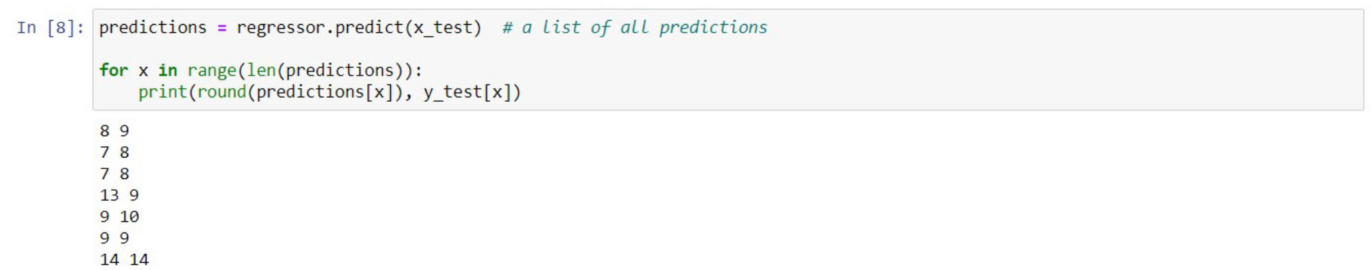
We see that most grade points are pretty close to the actual grades. For example, we predicted the first student’s final grade to be an 8 and it was 9.

Full code: Github Gist

You can try out different attributes in this dataset and see how well it improves or reduces the accuracy of the model.

Some Linear Regression Assumptions

1. Linearity: The relationship between X and y is linear.

2. No or little multicollinearity: Multicollinearity occurs when the independent variables are too highly correlated with each other.

3. Normality: For any fixed value of X, Y is normally distributed.

Other Real-Life Applications of Linear Regression

* Business: Predicting house prices with increases in the sizes of houses.

* Agriculture: Measuring the effect of fertilizer and water on crop yields.

* Healthcare: Predicting the impact of tobacco consumption and its association with heart disease.

Conclusion

Notice that we focused on the implementation of Linear Regression using Python’s Scikit-Learn library, and we didn’t go through any of the mathematical explanations to linear regression. To help, I have added really great tutorials to my resource list down below that explain the math behind Linear regression in the simplest way possible.

Resources:

[1] Python Machine Learning Playlist by Tech With Tim
[2] Linear Regression by Andrew Ng
[3] Linear Regression by StatQuest